Implicit Competitive Regularization
How do GANs generate?
Minimax is not enough
This post summarizes joint work with Anima and Hongkai. In the interest of conciseness, I will defer to our paper for discussions of related work and technical details. This Thursday July 16th at 9am and 8pm PDT, we will presenting our work at ICML2020.
GANs are fascinating! Not only can they generate strikingly realistic images, they also introduce an exciting new paradigm to mainstream machine learning.
Where ordinary neural networks learn by minimizing a fixed loss function, GANs consist of two neural networks that compete with each other in a zero-sum game. A generator produces fake images while a discriminator tries to distinguish them from real ones.
In most work on GANs, this is seen as the generator minimizing just another loss function that happens to be obtained by fully optimizing the discriminator.
I will argue that this minimax interpretation of GANs can not explain GAN performance. Instead, I believe that GAN performance can only be explained by the dynamics of simultaneous training.
In an attempt to make this more precise, I will explain how implicit competitive regularization (ICR) could allow GANs to generate good images. I will also provide empirical evidence that this is what actually happens in practice. Finally, I will use a game-theoretic interpretation of ICR to motivate the use of Competitive Gradient Descent (CGD) for the purpose of strengthening ICR. In our experiments on CIFAR 10, this leads to improved stability and higher inception score when compared to explicit regularization motivated by the minimax interpretation.
The GAN-dilemma
The objective function of the original GAN is
\[\min \limits_{\mathcal{G}} \max \limits_{\mathcal{D}} \mathbb{E}_{x \sim P_{\mathrm{data}}}\left[\log \left(\mathcal{D}(x)\right)\right] + \mathbb{E}_{z \sim \mathcal{N}}\left[\log \left( 1 - \mathcal{D}\left( \mathcal{G}\left(z\right)\right)\right)\right].\]Here, \(x \sim P_{\mathrm{data}}\) is sampled from the training data and \(z \sim \mathcal{N}\) from a multivariate normal. The generator network \(\mathcal{G}\) learns to map \(z\) to fake images and the discriminator network \(\mathcal{D}\) learns to classify images as real or fake.
If we take the maximum over all possible functions \(\mathcal{D}\), we obtain the Jensen-Shannon divergence (JSD) between the distributions of real and fake images. Therefore, it is believed that GANs work by minimizing the JSD between real and generated data. Subsequently, other GAN variants were proposed that are modeled after different divergences or metrics between probability distributions.
However, any such interpretation runs into one of the two following problems.
-
Without regularity constraints, the discriminator can (almost) always achieve perfect performance
-
Imposing regularity constraints needs a measure of similarity of images, which is hard to obtain.
We call this the GAN-dilemma.
Unconstrained discriminators can always be perfect
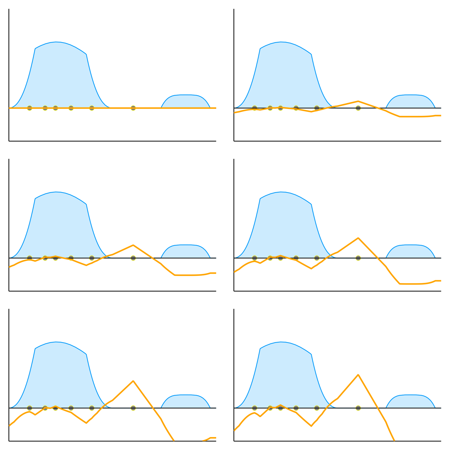
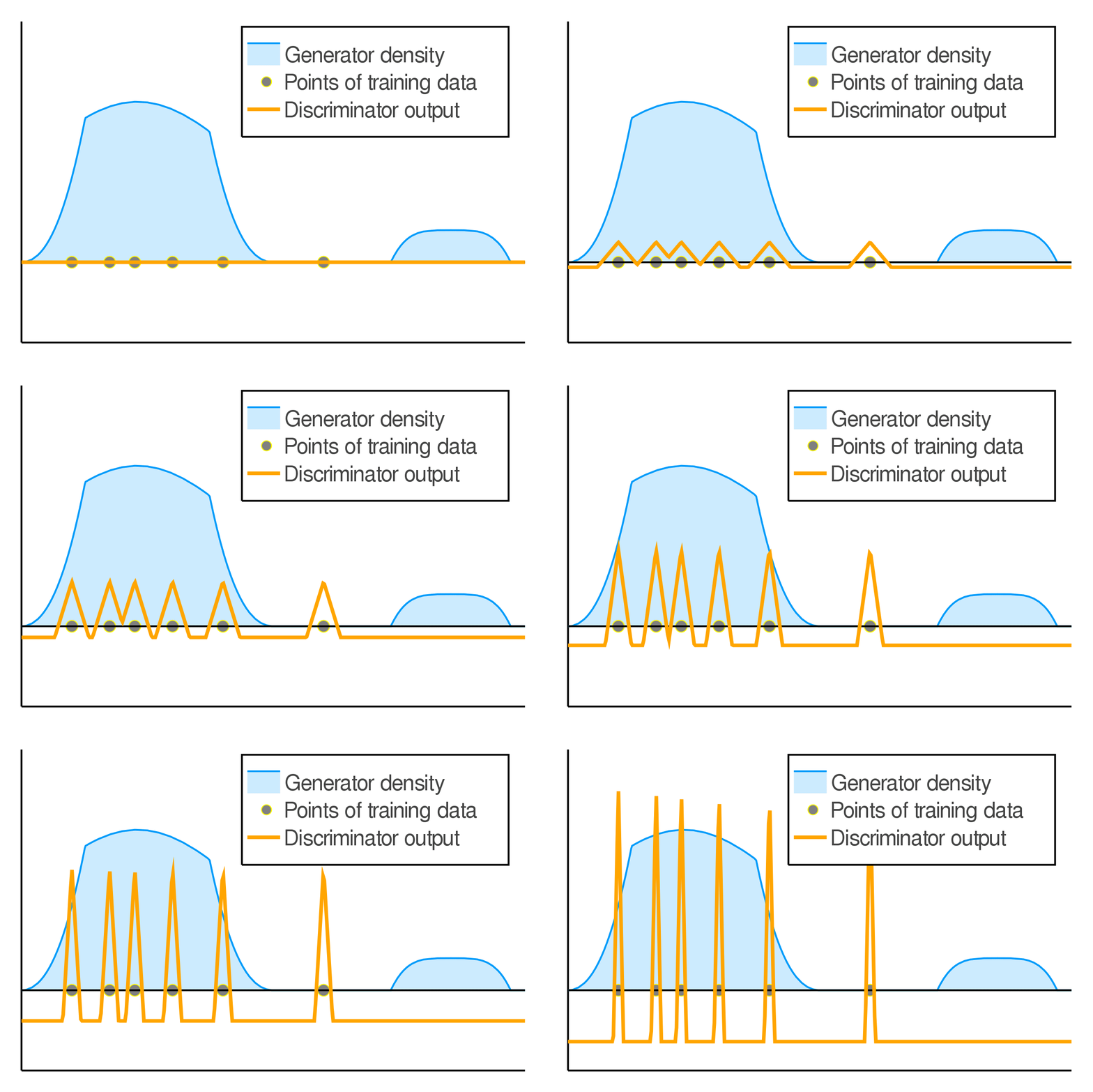
The original GAN falls into the first category. For instance, if we have a finite amount of training data and the generated distribution has a density, the discriminator can assign arbitrarily high values to the real data points, while assigning arbitrarily low values anywhere else.
Thus, for an optimal discriminator, the generator loss always has the same value. Therefore, it can not measure the relative quality of different generators.
Measuring visual similarity is hard!
This observation led to the development of WGAN, which instead uses (approximately) the formulation
\[\min \limits_{\mathcal{G}} \max \limits_{\mathcal{D}\colon \|\nabla \mathcal{D}\| \leq 1} \mathbb{E}_{x \sim P_{\mathrm{data}}}\left[\mathcal{D}(x)\right] - \mathbb{E}_{z \sim \mathcal{N}}\left[ \mathcal{D}\left( \mathcal{G}\left(z\right)\right)\right].\]The key difference here is the constraint on the discriminator. WGAN restricts the size of the gradient of the discriminator, forcing it to map nearby points to similar values. Thus, the generator loss under an optimal discriminator will be smaller if the generated images are closer to the true images. In fact, it will be equal to the earth mover’s distance between the two distributions.
The big catch is that we have to choose a way to quantify the size \(\left\| \nabla \mathcal{D}\right\|\) of the discriminator’s gradients! Since the inputs of the discriminator are images, this means we have to measure similarity of images.
Most variants of WGAN bound the Euclidean norm \(\left\| \nabla \mathcal{D}\right\|_2\) of the discriminator’s gradient. But this amounts to measuring the similarity of images by the Euclidean distance of the respective vectors of pixel-wise intensities. The example below shows that this is a terrible measure of visual similarity.

In general, quantifying visual similarity between images is a longstanding open problem in computer vision. Until this problem is solved we will not be able to meaningfully constrain the discriminator’s regularity.
A way out
In the above, I am not arguing that GANs cannot work. They work remarkably well! I am arguing that the minimax interpretation is but a red herring that has nothing to do with GAN performance.
Generative modeling is all about generating data similar to the training data. Since GANs can create realistic images, they must have access to a notion of image similarity that captures visual similarity. Most GAN variants can achieve good results, so this does not seem to be the result of a particular choice of loss function. Instead, it has to arise from the inductive biases of the neural network that parameterizes the discriminator.
Deep neural networks reliably learn patterns obvious to the human eye. This suggests that they capture something about visual similarity better than the feature maps, kernels, or metrics of classical computer vision.
The problem is that we cannot just open up the network to access this notion of similarity. Instead, it only arises implicitly, through the training process. In particular, the output of a neural network classifier on a sample does not reflect the uncertainty of the classification. This means that all information about how similar the fake images look to the real ones is lost once the discriminator is fully trained.
I think that the magic of GANs has to lie instead in the dynamics of simultaneous training that allows us to use the inductive biases of the discriminator for image generation, without explicitly characterizing them. I will now attempt to explain how this could be happening.
Implicit competitive regularization (ICR)
Simultaneous gradient descent (SimGD) has stable points that are unstable when only training one of the players with gradient descent, while keeping the other player fixed. We call this phenomenon implicit competitive regularization (ICR). For instance, we can consider the quadratic problem
\[\min \limits_x \max \limits_y x^2 + 10 xy + y^2\]and observe that SimGD with step sizes \(\eta_x = 0.09 , \eta_y = 0.01\) converges to \((0,0)\) even though this is the worst choice for the maximizing player. If we instead keep \(x\) fixed by setting \(\eta_x = 0\) and train \(y\) using gradient descent, it will diverge to infinity for almost all starting points.
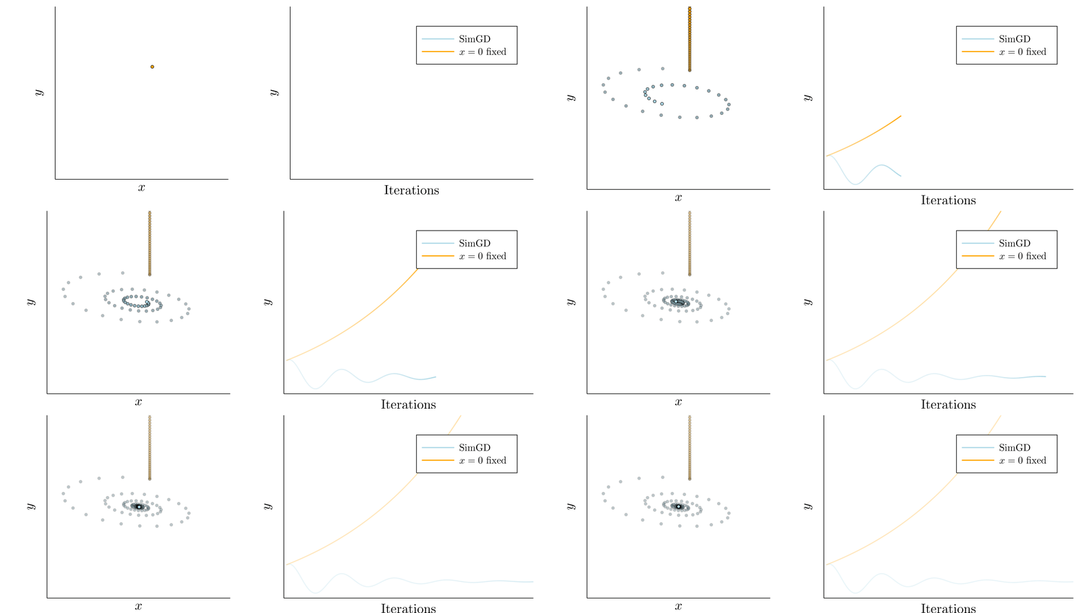
This is commonly seen as a flaw of SimGD, but I think it is crucial for GANs to work at all. Just like \(y\) can improve for any fixed \(x\), a GAN discriminator can improve for any fixed generator. Therefore, our only hope for convergent behavior in GANs is ICR!
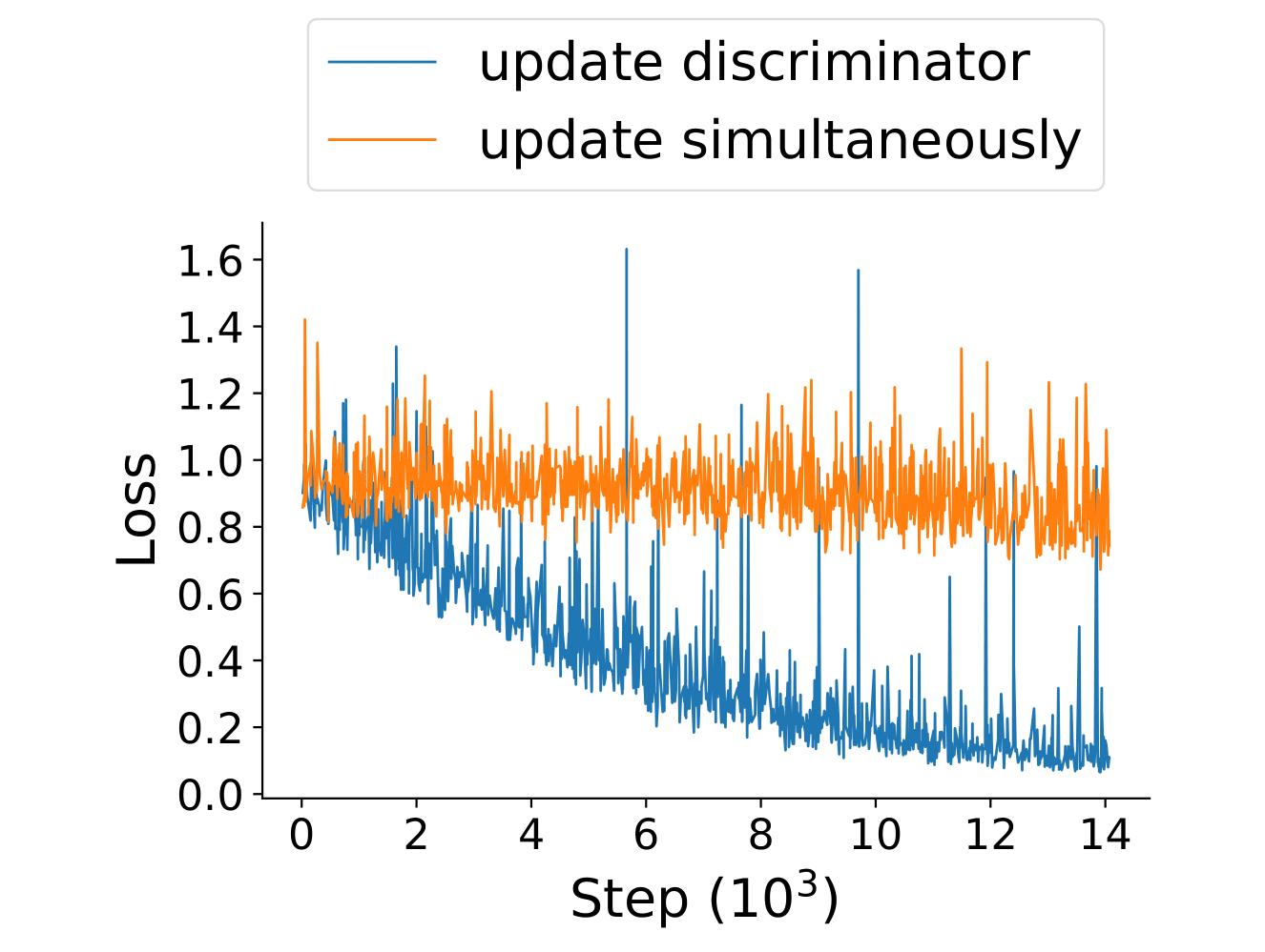
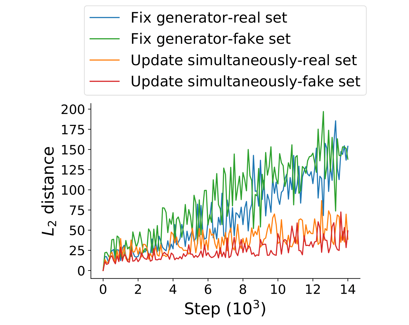
To verify this behavior in the wild, we train a GAN on MNIST until training stagnates and the generator produces good images. We then either train only the discriminator using gradient descent (keeping the generator fixed), or continue training both players using SimGD. We observe that the discriminator changes much more rapidly when trained in isolation, suggesting that the point of departure was indeed stabilized by ICR.
ICR selects for slowly learning discriminators
You might have noticed the peculiar choice of learning rates for the two players in the above example. This was no coincidence, but due to a fascinating property of ICR:
It selects for the relative speed of learning of \(x\) and \(y\)!
If we play around with the learning rate a bit more we notice that ICR is stronger if \(y\) (the player that would want to run off to infinity) learns slowly compared to \(x\).
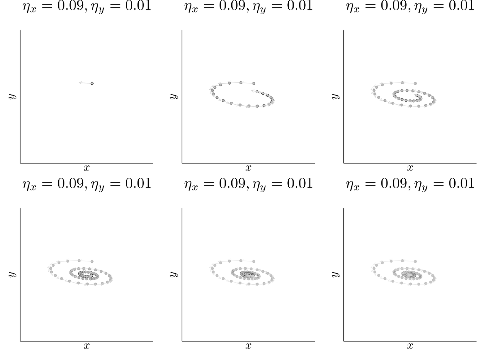
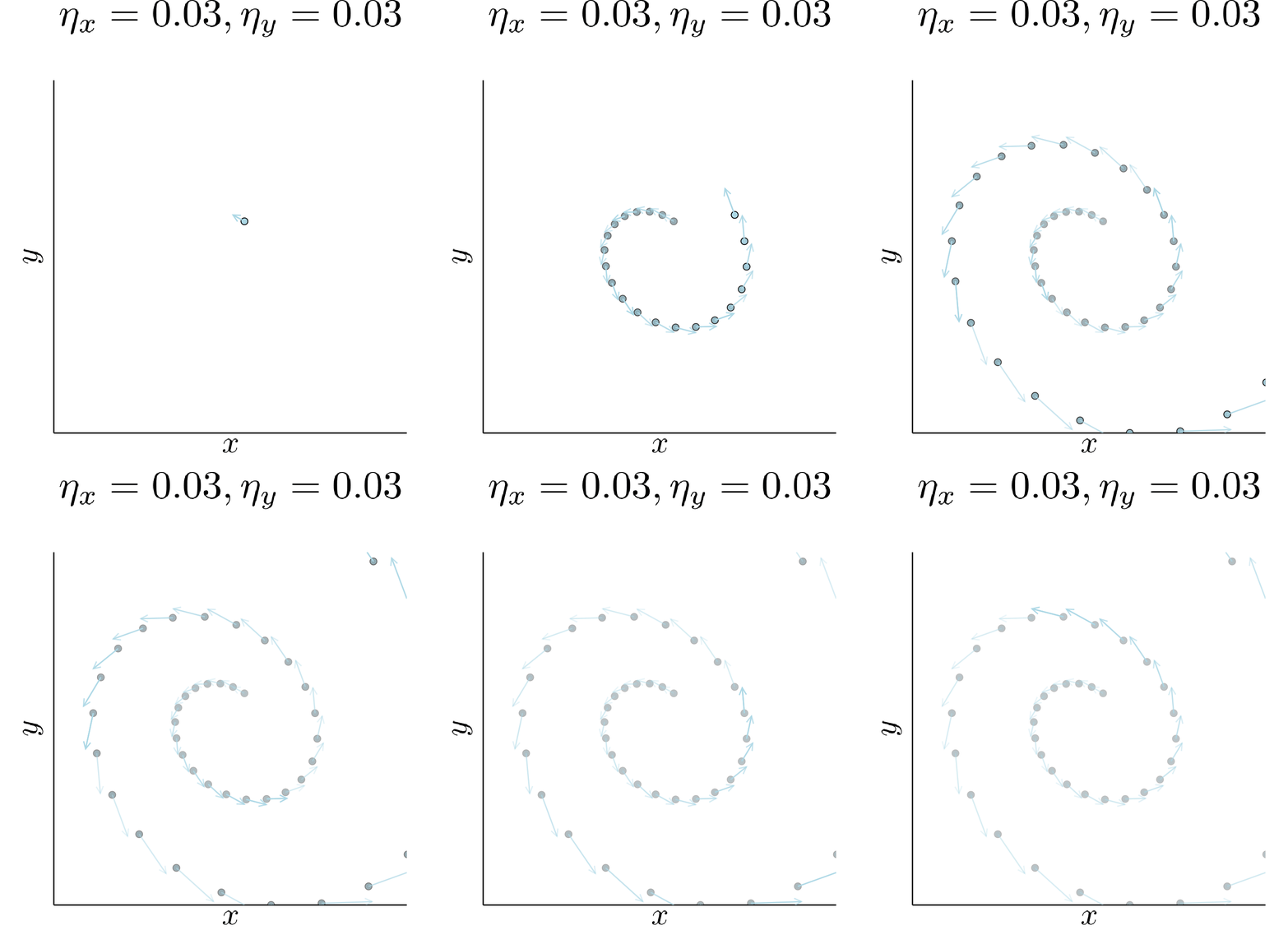
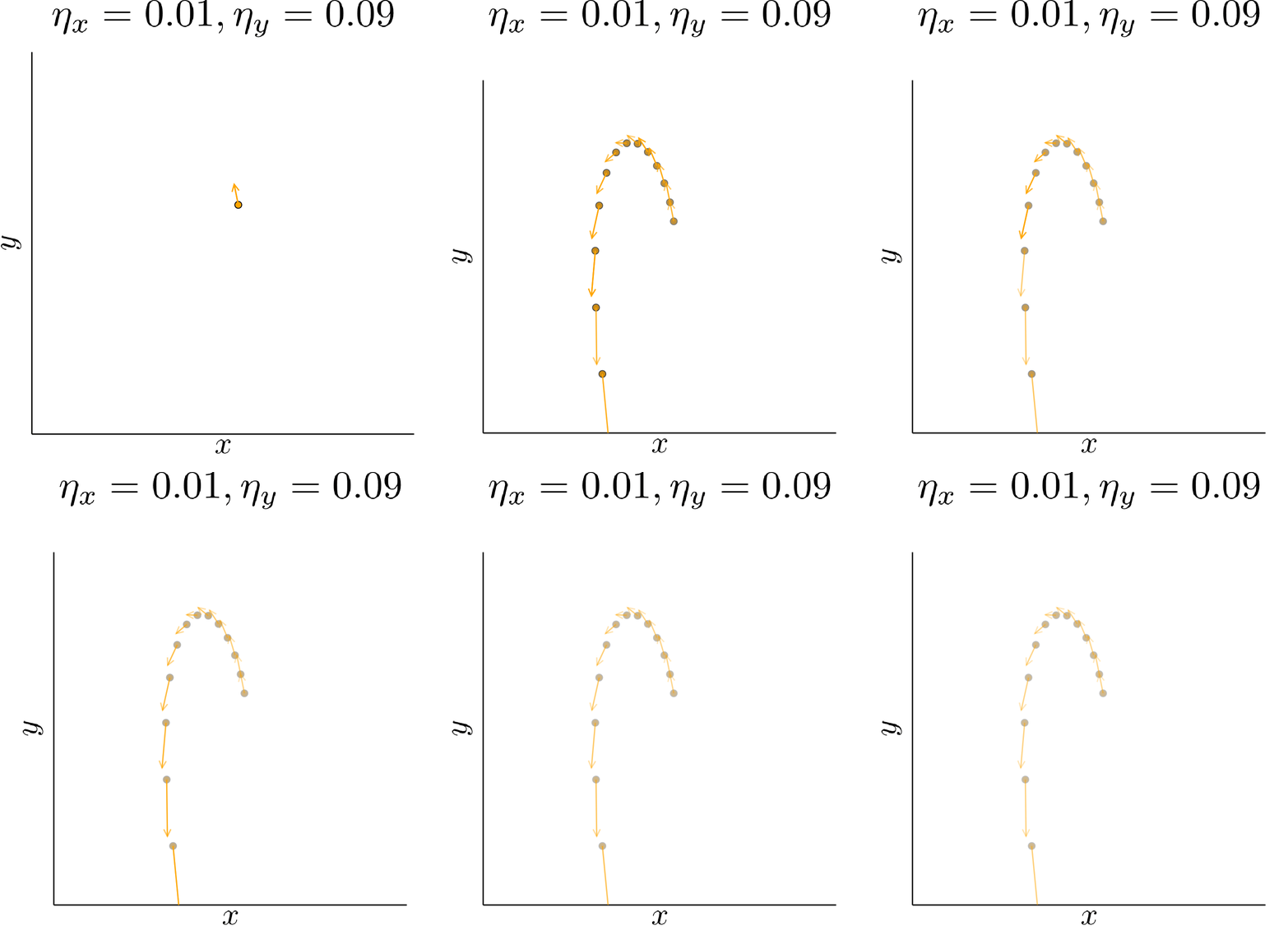
Our quadratic example has zero gradient only in \((0,0)\). Therefore, the presence of ICR only determines if we converge to it or not. A real GAN is highly nonlinear and has many points with vanishing gradient. ICR then determines to which of these points we can converge. In particular, out of all the critical points it will prefer points where the discriminator learns slowly.
What ICR has to do with image quality
We now have some idea about the kind of points that ICR stabilizes. But why should these points be good generative models?
Training and generalization even of “ordinary” deep neural networks is poorly understood. To address these questions in GANs, we will need to introduce a hypothesis of how the training dynamics of the discriminator relate to the quality of the input images.
Hypothesis: The speed with which the discriminator picks up on an imperfection of the generator measures the (human) visual prominence of the imperfection. Imperfections that are visually obvious will be picked up on more quickly than those that are visually subtle.
This hypothesis has not been rigorously verified, but it expresses the intuition that neural networks first learn simpler and more general patterns, before learning more intricate, specific ones. In this sense, it is also in line with the recently proposed coherent gradient hypothesis.
We have seen earlier that an unconstrained discriminator can always achieve perfect performance. The hypothesis says that how quickly it can do so measures the difficulty of the learning task. As we have seen, ICR can lead to convergence even if one player can achieve an infinite reward by running off to infinity, but only if this player learns slowly enough. Therefore we explain GAN performance with ICR selectively stabilizing points where the discriminator learns slowly. According to the hypothesis, these points are good generative models.
Implicit projection through ICR
Imagine there was a perceptual distance between distributions of images such that the discriminator learns more quickly to distinguish distant pairs of distributions than nearby ones. This distance measures similarity in the eyes of the discriminator, which by our hypothesis is a good proxy for similarity in the eyes of a human.
This distance would make for a great generator loss to use in a GAN, but unfortunately we can not compute it explicitly. Nevertheless, I will now show on a model problem how ICR could enable SimGD to use this distance for generative modeling.
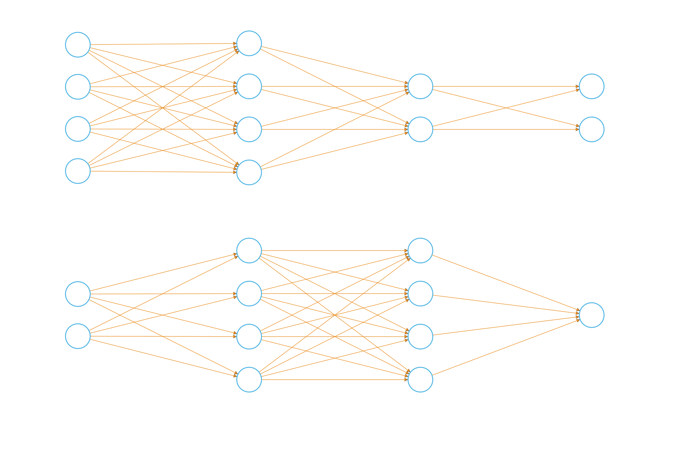
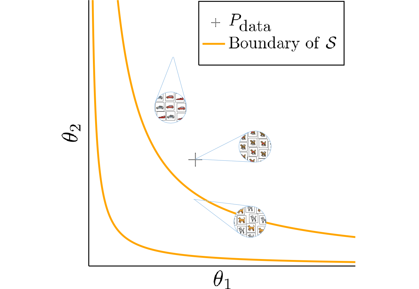
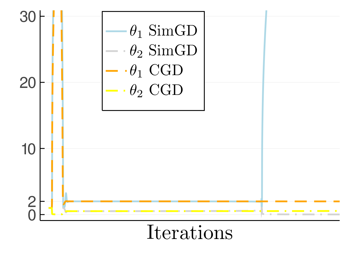
In our model problem, a “probability distribution” is characterized by two parameters, \(\theta_1\) and \(\theta_2\). The generator is a tiny neural network that maps its weights to a pair of parameters. It is parameterized such that it can only output distributions within the set \(\mathcal{S}\) that does not contain the true distribution \(P_{\mathrm{data}}=(2,2)\). Thus, it has to accept an error in at least one of the two parameters. The discriminator maps a set of weights and a pair of parameters to a real number.
It is hard to say how the perceptual distance of even such a simple network would look like. Therefore, we will model it explicitly by multiplying the discriminator input with a diagonal matrix \(\eta\) before feeding them to the network. We still can not characterize the perceptual distance exactly, but by changing the value of \(\eta\) we have some control over it. If for instance we choose \(\eta_{11} \gg \eta_{22}\), then the first component of the input images will lead to larger gradients. Thus, differences in the first component will be learned more quickly and contribute more to the perceptual distance.
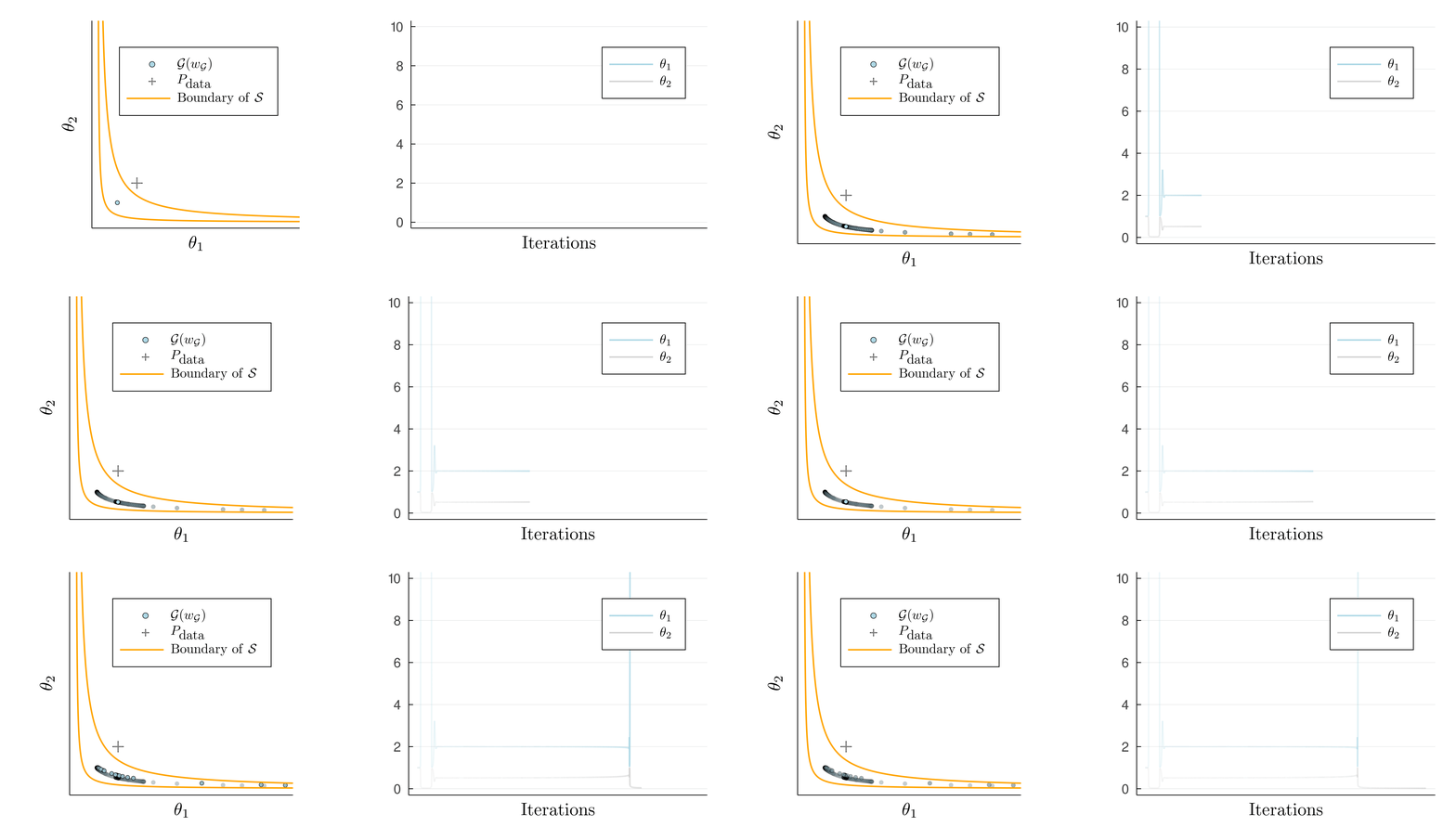
Setting \(\eta_{11} = 10^2, \eta_{22} = 1\) we would like the generator to accept some error in the second component for the sake of getting the first component right. But we cannot characterize the perceptual distance explicitly, so this will have to happen without us explicitly using \(\eta\).
Amazingly, SimGD solves this problem for us! If we train networks using SimGD, the generator will spend long periods of time getting the first component right, while accepting an error in the second one. We have used SimGD to compute a projection with respect to the perceptual distance without knowing it.
Improving GAN training by strengthening ICR
The implicit projection does not last forever and eventually the system snaps out and diverges. Similarly, our GAN example on MNIST had not fully converged and kept changing even when using SimGD. This suggests that ICR is too weak to permanently stabilizes the system. Instead, it merely slows down divergence by forcing the GAN to slowly spiral away, rather than diverge on a straight path.
The instability of GAN training is a huge problem in practice that needs to be overcome by careful selection of hyperparameters. Since GAN performance is hard to quantify, this requires tedious manual labor on top of a huge computational budget.
Since we believe that ICR is at the center of GAN performance, we want to stabilize training by strengthening ICR instead of just adding generic regularizers like dropout, weight decay, or spectral regularization to the network. To this end, it will be instructive to have a game-theoretic look at ICR.
A game perspective on ICR
Consider again our quadratic example
\[\min \limits_x \max \limits_y x^2 + 10 xy + y^2.\]We have seen that SimGD can converge to \((0,0)\) on this problem, for suitable step sizes. This is strange, since we think of SimGD as both players greedily improving their objective and for every fixed value of \(x\), the best thing for \(y\) would be to run off to infinity as quickly as possible.
To understand what is going on assume we start in \((x,y) = (0,1)\). The gradient of \(y\) points towards \(\infty\), making it move to \(1 + \delta\) for some \(\delta > 0\). At the same time, the gradient of \(x\) points towards \(-\infty\), making it move to \(-\epsilon\), for some \(\epsilon > 0\). If \(x\) had stood still, the move of \(y\) had decreased its loss from to \(-1^2\) to \(-(1 + \delta)^2\). But because of the actions of \(x\), \(y\)’s move incurs an additional loss of \(10 \epsilon \delta\). This can be interpreted as \(y\)’s move exposing it to counterattack by \(x\). If \(x\) moves quickly enough meaning that \(\epsilon\) is large enough, this mixed term will incentivize \(y\) to move back towards zero. This is the mechanism underlying ICR.
Thus, ICR arises because the players try to avoid exposing themselves to counterattack of their opponents.
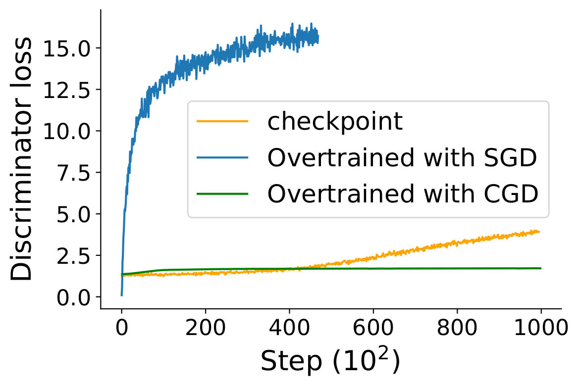
Remember our example on MNIST where we only trained the discriminator while keeping the checkpoint generator fixed. The discriminator was able to greatly decrease its loss, but what if we allow the generator to fight back.
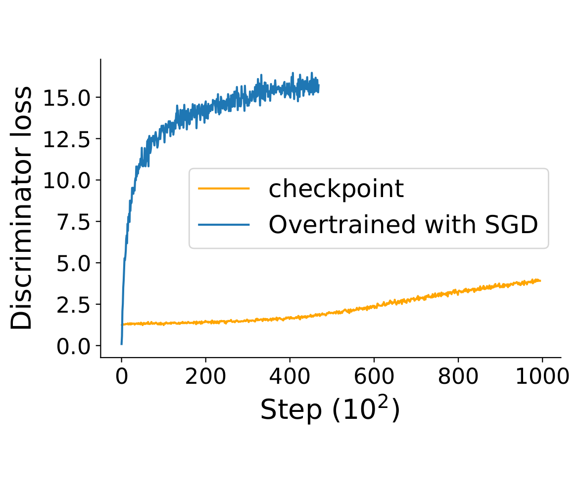
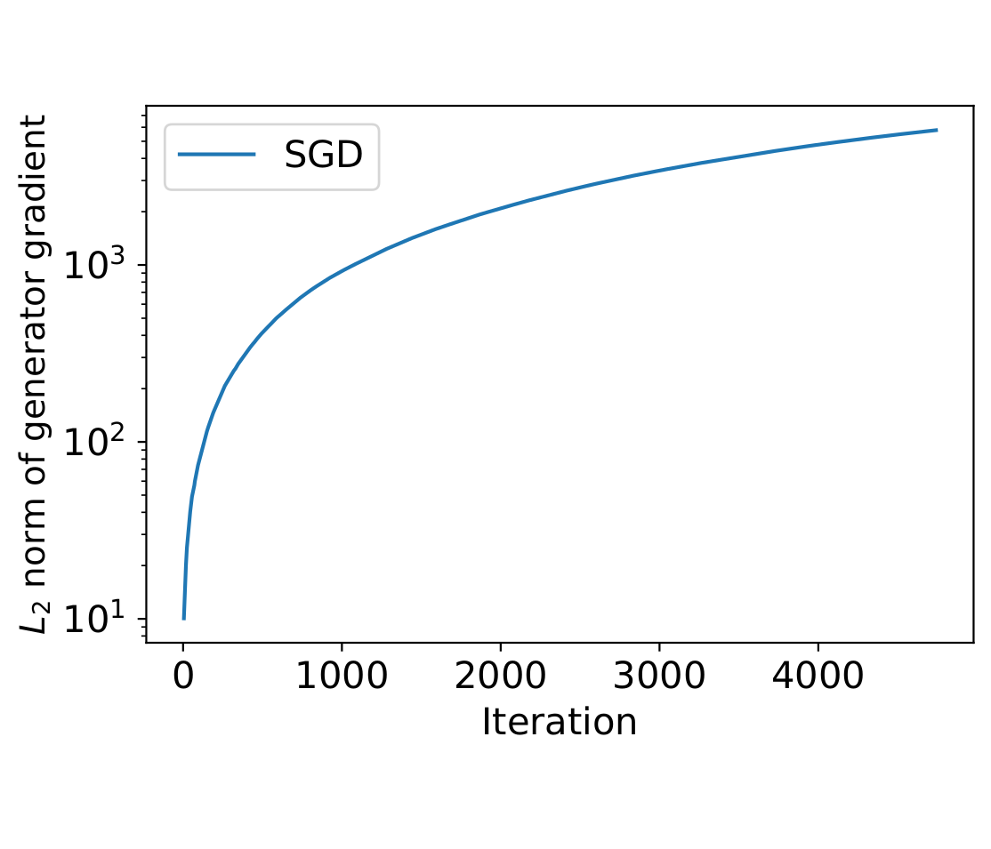
BOOM! As soon as the generator is allowed to move, the discriminator loss skyrockets. The decreased loss was only achieved at the expense of brittleness to counterattack.
Competitive gradient descent for stronger ICR
As described above, ICR can be interpreted as arising from the agent’s desire to be robust to counterattack. However, under SimGD they do not take the presence of their opponent into account while making their decision.
In the quadratic example above, \(y\) starts to feel the presence of \(x\) only once \(x\) has moved to \(\epsilon\). Depending on the step size, this delay can be enough for the system to become unstable. This is also the reason why, infamously, SimGD applied to the the bilinear loss \((x,y) \mapsto xy\) does not converge to the Nash-equilibrium in \((0,0)\).
If \(y\) were aware of its opponent while making its decision it could have anticipated \(x\)’s actions and directly moved to \(1-\delta\) to mitigate its impact. Algorithmically, this results in greater stability of the point \((0,0)\).
Competitive Gradient Descent (CGD) lets both players try to anticipate each other’s action by solving for a local Nash-equilbrium at every step, which results in greatly increased ICR.
When applying CGD to the example on MNIST, we see that training the discriminator using CGD while keeping the generator fixed will make it even more robust to counteraction of the discriminator. We also observe that CGD prolongs the duration of the projection state in the example on ICR
Experiments on CIFAR 10
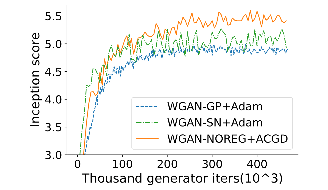
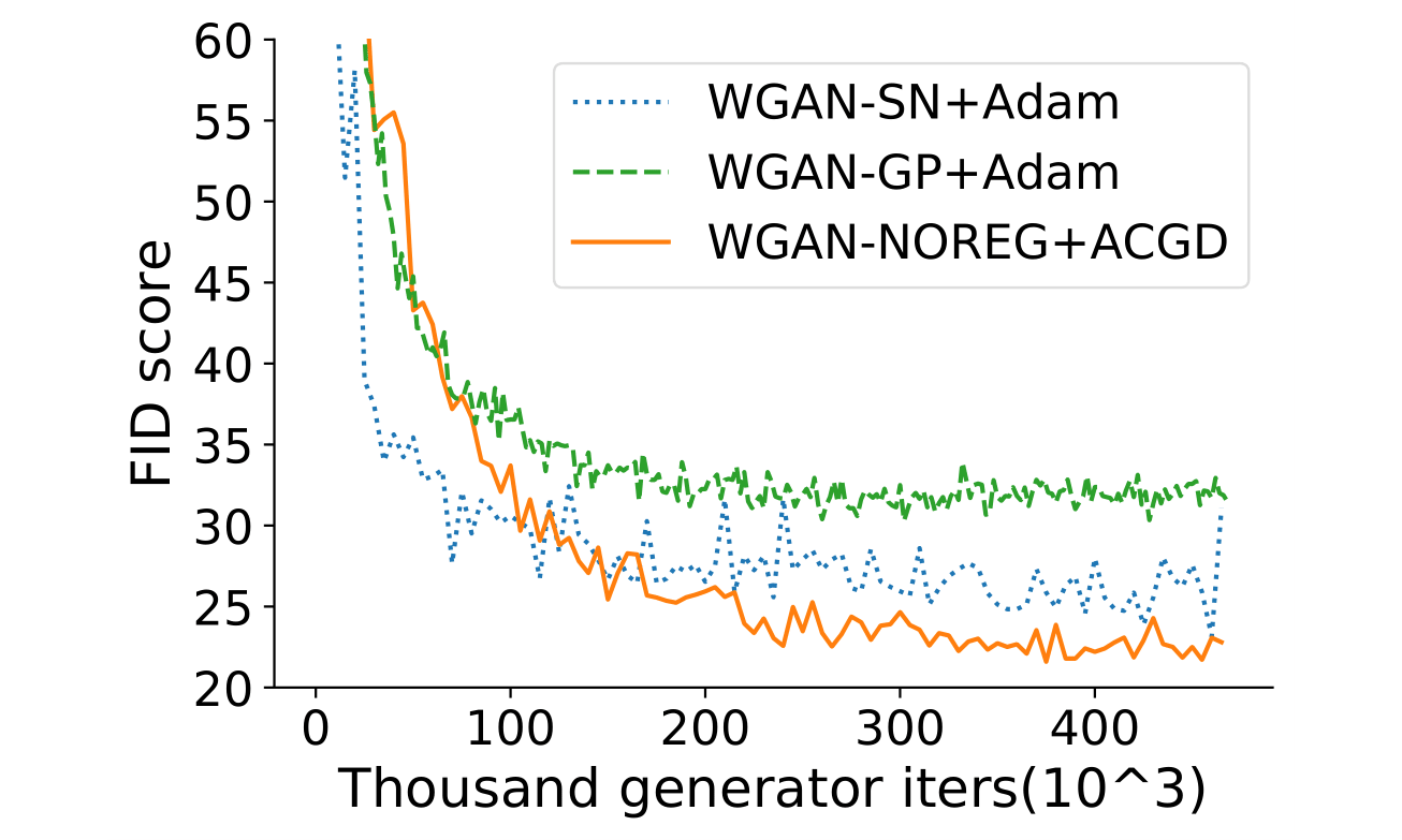
Based on the above, we hoped that strengthening ICR by training GANs with CGD would lead to better results than explicit regularization through, for instance, gradient penalties. To this end, we used the same DCGAN-architecture as in WGAN-GP and combined different regularizers and loss function. Indeed, we find that training with ACGD (CGD combined with an RMSProp-type heuristic) yields better and more consistent results, as measured by the inception score (IS) and Fréchet inception distance. We see this as additional evidence that ICR is a key element of GAN performance.
Conclusion
Instead of scrambling to salvage the minimax point of view, I think that it is more practical and more interesting to embrace the fact that these algorithms are designed as an iterative game and do not amount to a single player implicitly minimizing a loss function.
This requires us to better understand why points found by adversarial training should be useful for a given downstream task.
I hope that the work outlined above will pave the way for a better understanding of adversarial training. In the long run, I believe that this will greatly expand the range of problems that can be solved using deep neural networks.
