Sparse factorization of dense matrices

Fade-out instead of fill-in

Introduction

This post summarizes joint work with Tim and Houman on the sparse Cholesky factorization of dense kernel matrices. In the interest of conciseness, I will defer to our paper for discussions of related work and technical details.

Kernel Matrices

Positive definite kernel matrices of the form

\[\Theta_{ij} := \mathcal{G}\left(x_i, x_j\right)\]

play an important role in many parts of computational mathematics. They arise as covariance matrices of Gaussian processes in statistics and as discretized solution operators of partial differential equations in computational engineering. By means of the kernel trick, they allow machine learning algorithms to employ infinite dimensional features maps.

(Finitely) smooth Gaussian processes

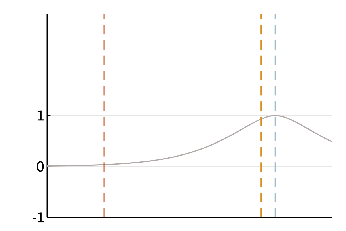
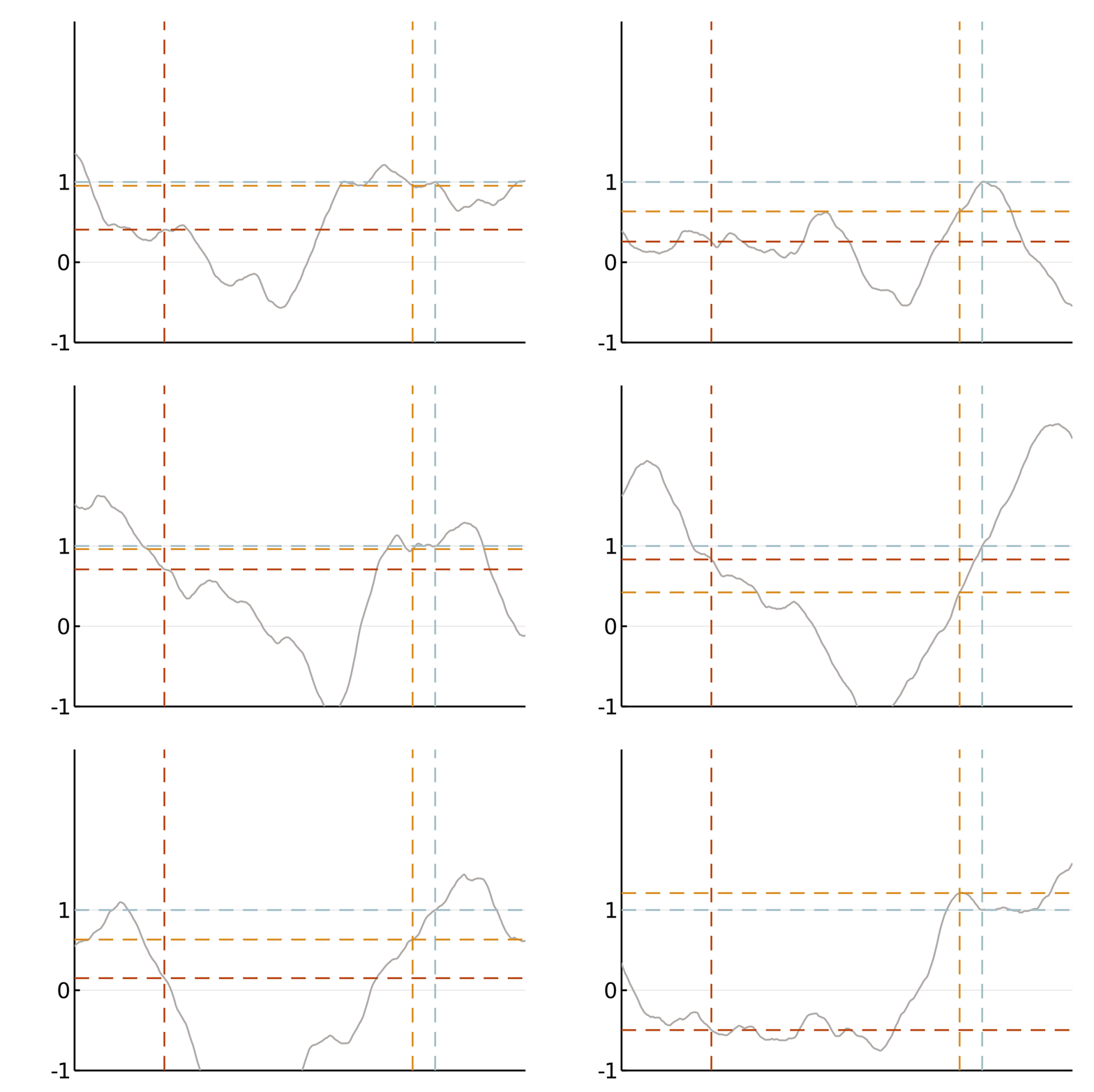
We focus on covariance matrices of finitely smooth Gaussian processes or, equivalently, the solution operators of elliptic partial differential equations (PDEs). Qualitatively, these kernels assign larger values to pairs of nearby points and smaller values to pairs of distant points. This means that if we observe a smooth random process to be positive in a point $x$, we will strongly expect it to be positive at a nearby point $y$. If this is all we know, we also tend to believe that values at a more distant point $z$ are positive, but we will be less confident in this belief. A popular class of such covariance functions is given by the Matérn family.

The correlation is positive and falls of with distance

Nearby points have similar values, values of more distant points become less dependent.

On the left we show the correlation between values at $ {\color{#A1BDC7} x } $ and other points under a Matérn model. On the right we show different realizations of the assoe ciated Gaussian process, conditioned to be one in $ {\color{#A1BDC7} x } $. The values at the nearby point $ {\color{#D98C21} y} $ are close to one. The values at the distant point $ {\color{#B8420F} z} $ are positive on average, but vary wildly.

The cubic bottleneck

In most applications, we need to apply a kernel matrix to a vector ($v \mapsto \Theta v$), apply its inverse to a vector ($v \mapsto \Theta^{-1}v$), or compute its logdeterminant. However, $\Theta$ is usually dense, meaning that most of its entries are not small enough to be ignored. When using $N$ points of data, even storing the matrix has complexity $N^2$ and inverting it using a dense Cholesky factorization has complexity $N^3$. This becomes the major computational bottleneck in contemporary problems featuring large amounts of data and complex physical models.

Our method

We improve the state of the art computational efficiency by a simple three step algorithm.

Reorder the degrees of freedom, and therefore the rows and columns of $\Theta$.
Compute the entries of $\Theta$ on a sparsity set $\mathcal{S}$ of just near-linearly many entries.
Compute the Cholesky factorization $\Theta$, ignoring any operations outside of $\mathcal{S}$.

Picking the ordering

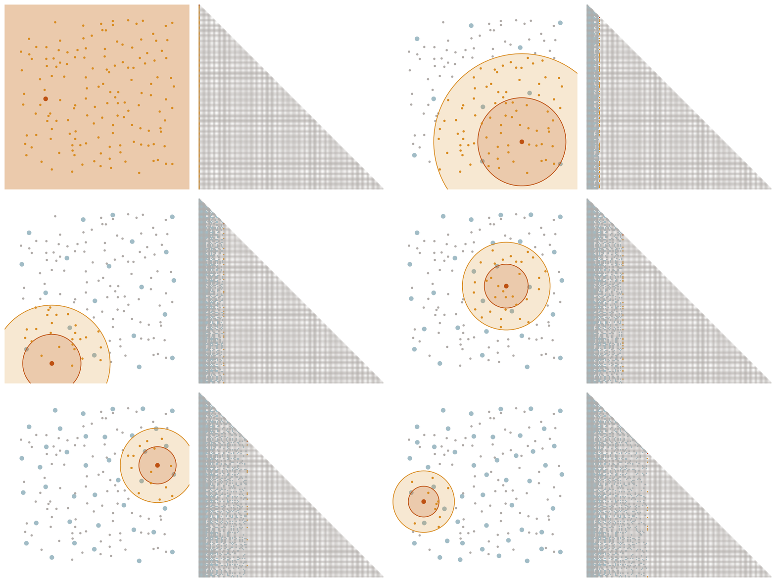
We order the datapoints from coarse to fine according to the maximin ordering. This means that we successively pick the point that is furthest away from the points that we have picked already, starting with an arbitrary point.

Selecting the sparsity set

We denote as $\ell_i$ the distance that the $i$-th point of the maximin ordering had to the points picked before. We choose a tuning parameter $\rho$ and let $x_i$ interact with all points later in the ordering that have a distance at most $\rho \ell_i$. This means that we add an element $(i,j)$ to the sparsity set $S_\rho$ if $i \geq j$ and $\mathrm{dist}(x_i, x_j) \leq \rho \ell_i$.

Incomplete Cholesky factorization

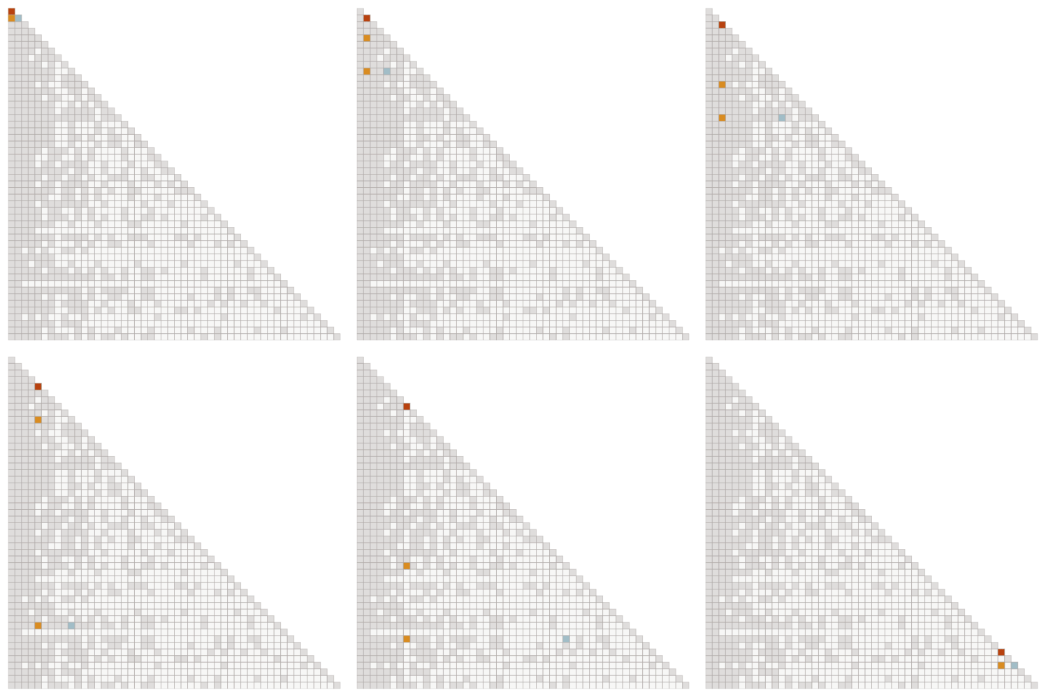
The Cholesky factorization takes in the lower triangular part of a Matrix $\Theta$ and, by updates of the form $\Theta_{ki} \leftarrow \Theta_{kj} - \Theta_{ki} \Theta_{ji} / \Theta_{ii}$, transforms it into a lower triangular matrix $L$ that satisfies $L L^{\top} = \Theta$. We exploit the sparsity of $S_\rho$ by instead computing the incomplete Cholesky factorization that treats entries outside of $S_\rho$ as zero and skips updates involving them.

We select an ordering and sparsity pattern

and then compute the incomplete Cholesky factorization.

The maximin ordering successively selects the point $ {\color{#B8420F} x_k} $ that has maximal distance $ {\color{#B8420F} \ell_k} $ from the points that were selected so far (left). We add those entries corresponding to interactions of $ {\color{#B8420F}x_k} $ with points within radius $ {\color{#D98C21}\rho \ell_k} $ to the sparsity pattern $ {\color{#A1BDC7} S_\rho} $ (middle). We then compute the incomplete Cholesky factorization, meaning that we skip the update $ {\color{#A1BDC7}\Theta_{kj}} \leftarrow {\color{#A1BDC7} \Theta_{kj}} - {\color{#D98C21} \Theta_{ki} \Theta_{ji}} / {\color{#B8420F}\Theta_{ii}} $ whenever it involves entries outside the sparsity pattern (right).

Sparsity allows for fast computation

If the set $\{x_i\}_{1 \leq i \leq N}$ is $d$-dimensional, this can be done in time $\mathcal{O}\left(N \log^{2}\left(N\right) \rho^{2d} \right)$ and space $\mathcal{O}\left(N \log^{}\left(N\right) \rho^{d} \right)$. This yields a major improvement over the naive complexity $\mathcal{O}(N^3)$.

It works! But why?

The algorithm described above produces a sparse lower triangular matrix $L$ that approximates the kernel matrix as $L L^{\top} \approx \Theta$. Due to being triangular, $L$ and $L^{\top}$ can be inverted efficiently using forward and back substitution and their determinant the product of their diagonal entries.

Exponential accuracy

But how accurate is $L L^{\top} \approx \Theta$. We have performed two very aggressive approximations: First we have set all but $\mathcal{O}\left(N \log\left(N\right) \rho^{d} \right)$ many entries of the dense $N \times N$ matrix $\Theta$ to zero, and then we have skipped all but $\mathcal{O}\left(N \log^{2}\left(N\right) \rho^{2d} \right)$ operations of its Cholesky factorization. By itself, either of these approximations results in a horrible approximation error. But in combination they provide an accurate approximation. In fact, we prove that if $\Theta$ is the Green’s matrix of an elliptic boundary value problem and $\rho \approx \log(N)$, we get $\log\left(\left\|\Theta - L L^{\top}\right\| \right) \lesssim -\rho$. The error decays exponentially in $\rho$!

Fade-out instead of fill-in

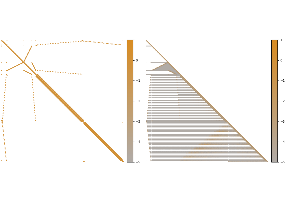
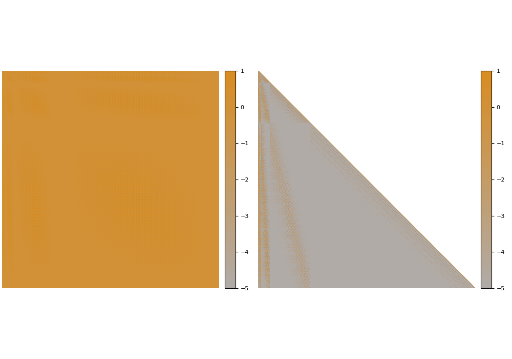
The Cholesky factorization of sparse matrices is a classical field in numerical analysis. In this case, the main difficulty is dealing with fill-in that leads to Cholesky factors that are much denser than the input matrix. In contrast, we observe that many dense kernel matrices exhibit fade-out, leading to almost sparse Cholesky factors.

Gaussian elimination and Gaussian processes

The fade-out phenomenon has not been observed before but from a probabilistic point of view it is not surprising. Cholesky factorization can be interpreted as recursive application of

$$ \begin{pmatrix} \Theta_{1,1} & \Theta _{1,2} \\ \Theta_{2,1} & \Theta_{2,2} \end{pmatrix} = \begin{pmatrix} \mathrm{Id} & 0 \\ {\color{#D98C21} \Theta_{2,1}\left(\Theta_{1, 1}\right)^{-1}} & \mathrm{Id} \end{pmatrix} \begin{pmatrix} \Theta_{1, 1} & 0 \\ 0 & {\color{#A1BDC7} \Theta_{2,2} - \Theta_{2,1} \left(\Theta_{1,1}\right)^{-1} \Theta_{1,2}} \end{pmatrix} \begin{pmatrix} \mathrm{Id} & {\color{#D98C21} \left(\Theta_{1, 1}\right)^{-1}\Theta_{1,2}}\\ 0 & \mathrm{Id} \end{pmatrix}. $$

For $(X_1, X_2) \sim \mathcal{N}\left(0, \Theta\right)$ we have

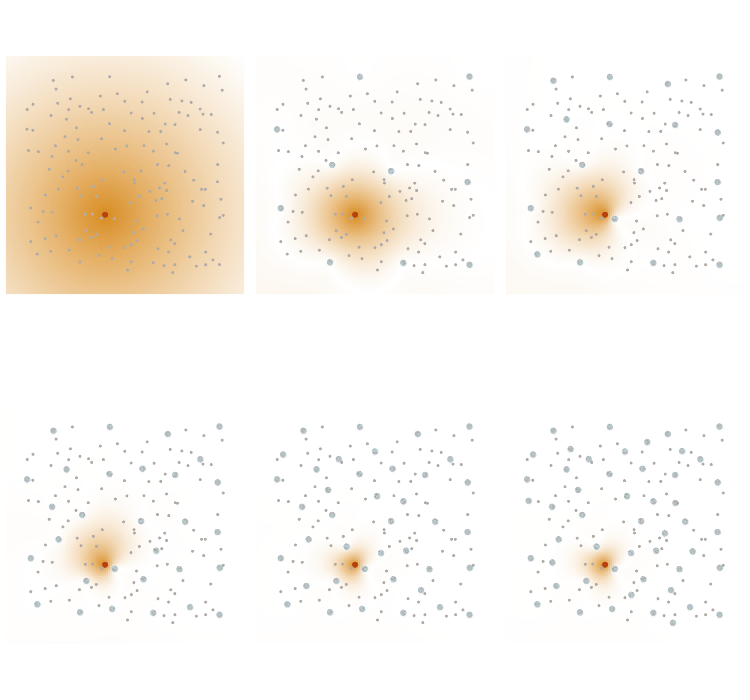
\[\mathbb{E}\left[ X_2 \middle| X_1 = a \right] = {\color{#D98C21}\Theta_{2,1}\left(\Theta_{1, 1}\right)^{-1}} a \quad \mathrm{and} \quad\mathrm{Cov}\left[X_2 \middle| X_1 \right] = {\color{#A1BDC7}\Theta_{2,2} - \Theta_{2,1} \left(\Theta_{1,1}\right)^{-1} \Theta_{1,2}}\]

meaning that Cholesky factorization amounts to iteratively conditioning a Gaussian process. In particular, conditional independence in the Gaussian process $X$ directly corresponds to sparsity in the Cholesky factors of $\Theta$. There are many interesting densely correlated stochastic processes that feature conditional independence. Therefore, many interesting dense matrices are subject to fade-out.

Many sparse matrices exhibit fill-in, leading to dense Cholesky factors

In contrast, we show that some dense matrices feature fade-out, leading to sparse Cholesky factors

It is well known that many sparse matrices exhibit fill-in, leading to substantially dense Cholesky factors. (left) In contrast, we observe that the dense covariance matrices of smooth Gaussian processes exhibit fade-out, leading to almost sparse Cholesky factors. (center, magnitude of entries on $ \log_{10} $ scale). This behavior is due to the screening effect, whereby the conditional correlation of a given point will localize, as we condition on nearby points (right).

The screening effect

In the case of covariance matrices of finitely smooth Gaussian processes, the sparsity of their Cholesky factors is predicted by the screening effect. We have seen in the introduction that the values at a point $y$ close to $x$ are much more informative of the value at $x$ than those at a distant point $z$. This means that the value at $x$ is almost independent of that at $z$, conditional on the value at $y$. Under the elimination ordering chosen in our method, the first $k$ points cover the data set up to a distance $\ell_k$. Conditional on the values at these points, the correlation length is of the order $\ell_k$, which informs our choice of sparsity pattern $S_\rho$.

Wrapping up

Cholesky factorization and the numerical analysis of elliptic partial differential equations are classical field of applied mathematics. Nevertheless, the probabilistic intuition described above leads to a simple algorithm that improves the state of the art computational complexity on a large class of problems. In our paper, we draw connections to operator adapted wavelets and numerical homogenization that allow us to prove these results rigorously. There, we also show that incomplete Cholesky factorization in the reverse maximin ordering allows to efficiently invert the sparse stiffness matrices of elliptic PDEs. Just like in the case of Green’s matrices, this simple algorithm improves upon the state of the art computational complexity for general elliptic PDEs. Furthermore, our methods allow for the efficient computation of near optimal low-rank approximations, corresponding to the principal component analysis (in the Green’s matrix case) or homogenization (in the stiffness matrix case). In recent follow-up work, we extend these ideas to provide an embarassingly parallel algorithm with even better computational complexity.