Competitive Gradient Descent
Gradient descent for multi-player games?
Introduction
This post summarizes joint work with Anima on a new algorithm for competitive optimization: Competitive gradient descent (CGD). If you want to know more, you should check out the paper or play with Hongkai’s pytorch code.
Many learning algorithms are modelled as a single agent minimizing a loss function, such as empirical risk. However, the spectacular successes of generative adversarial networks (GANs) have renewed interest in algorithms that are modeled after multiple agents that compete in optimizing their own objective functions, which we refer to as competitive optimization.
Since much of single agent machine learning is powered by variants of gradient descent, this raises the important question: What is the natural generalization of gradient descent to competitive optimization? In this note, I will try to convince you that this natural generalization of gradient descent is a novel algorithm, with a beautiful game-theoretic interpretation and promising practical performance.
The problem with simultaneous gradient descent
Consider a single-agent optimization problem, \(\min_{x \in \mathbb{R}^{m}} f(x).\) Gradient descent (GD) with step size \(\eta\) is given by the update rule
\[x_{k+1} = x_{k} - \eta \nabla f(x_{k})\]where the gradient \(\nabla f(x_{k})\) is the vector containing the partial derivatives of \(f\), taken in the last iterate \(x_k\). The vector \(-\nabla f(x_{k})\) points in the direction of the steepest descent of the loss function \(f\) in the point \(x_k\), which is why gradient descent is also referred to as the method of steepest descent.
Let us now move to the competitive optimization problem:
\[\min \limits_{x \in \mathbb{R}^m} f(x, y)\] \[\min \limits_{y \in \mathbb{R}^n} g(x, y)\]restricting ourselves to two agents for the sake of simplicity. Here, the first agent tries to choose \(x\) such as to minimize \(f\), while the second agent tries to choose the decision variable \(y\) such as to minimize \(g\). The interesting part is that the optimal choice of \(x\) depends of \(y\) and vice versa, and the objectives of the two players will in general be at odds with each other, the important special case \(f = -g\) corresponding to zero-sum or minimax games.
Since neither player can know what the other player will do, they might assume each other to not move at all. Under this assumption, following the direction of steepest descent seems like a reasonable strategy, leading to simultaneous gradient descent (SimGD).
\[x_{k+1} = x_{k} - \eta \nabla_x f(x_{k}, y_{k})\] \[y_{k+1} = y_{k} - \eta \nabla_y f(x_{k}, y_{k}).\]Here, \(\nabla_x f(x_{k}, y_{k}) \in \mathbb{R}^m\) and \(\nabla_y f(x_{k}, y_{k}) \in \mathbb{R}^n\) denote the gradient with respect to the variables \(x\) and \(y\), respectively.
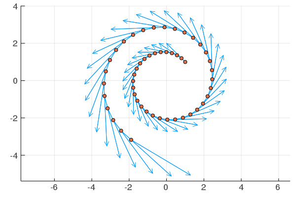
Unfortunately, even on the most simple bilinear minimax problem \(f(x,y) = x^{\top} y = - g(x,y)\), SimGD fails to converge to the Nash equilibrium \((0,0)\). Instead, its trajectories form ever larger cycles as the two players chase each other in strategy space. The oscillatory behavior of SimGD is not restricted to this toy problem and a variety of corrections have been proposed in the literature.

Gradient descent revisited
Rather than adding modifications to SimGD, we begin by revisiting gradient descent. It is well-known that the GD update can equivalently be written as
\[x_{k+1} = \arg \min \limits_{x \in \mathbb{R}^m} f(x_{k}) + Df(x_{k}) (x - x_{k}) + \frac{1}{2 \eta} \|x - x_{k}\|^2.\]Here, \(Df(x_{k}) = (\nabla f(x_{k}))^{\top}\) is the \(1 \times m\)-matrix containing the partial derivatives of \(f\). This can be interpreted as the agent the linear approximation in the last iterate, \(x \mapsto f(x_{k}) + Df(x_{k}) (x - x_{k})\), adding a quadrative regularization term that expresses her distrust of this approximation far away form the point of linearization. This suggests that for multiple players, the gradient descent update should be the solution of a local first order approximation of the full problem, with quadratic regularization terms on each player that express their limited confidence in this approximation.
Linear or bilinear
This begs a fundamental question: What is the right notion of local first order approximation for multi-agent optimization problems?. In single-agent optimization, the local first order approximation of the problem is obtained as the linear approximation of the objective functions. If we use a linear approximation of both agents’ loss function, we obtain the following game.
\[\min \limits_{x \in \mathbb{R}^m} \ f + D_{x}f (x-x_k) + D_{y}f(y - y_k) + \frac{1}{2 \eta}\|x - x_k\|^2\] \[\min \limits_{y \in \mathbb{R}^n} \ g + D_{x}g (x-x_k) + D_{y}g(y - y_k) + \frac{1}{2 \eta}\|y - y_k\|^2.\]Here and in the following, the evaluations of loss functions and their derivatives always occur in the last iterate \((x_k, y_k)\), unless otherwise mentioned. When looking at the above local game we observe that the optimal strategy of player \(x\) is independent of \(y\) and vice versa. Thus, the above game is equivalent to
\[\min \limits_{y ∈ \mathbb{R}^m} f + D_{x}f (x-x_k) + \frac{1}{2 \eta}\|x - x_k\|^2,\] \[\min \limits_{x ∈ \mathbb{R}^n} g + D_{y}g(y - y_k) + \frac{1}{2 \eta}\|y - y_k\|^2,\]which leads to the update rule of SimGD. One explanation for the poor convergence properties of SimGD is that the underlying local game has completely lost the underlying game-theoretic structure and instead consists of both players myopically minimizing their own objective function.
Instead of generalizing the linear approximation in the single-agent case to a linear approximation in the multi-agent case, we could also generalize it to a multilinear approximation. Instead of using polynomial terms up to first order (\(f\), \(g\), \(D_x f\), \(D_y f\), \(D_x g\), \(D_y g\)) we use use derivatives up to first order per agent. In the two-agent setting, this is the bilinear approximation obtained by including the “mixed” second derivatives (\(D_{xy}^2f\), \(D_{yx}f^2\), \(D_{xy}^2g\), and \(D_{yx}^2g\)) in the approximation, while omitting the “pure” second derivatives (\(D_{xx}^2f\), \(D_{yy}^2f\), \(D_{xx}^2g\), and \(D_{yy}^2g\)). The resulting local game is
which can be simplified to
This local game preserves the interactive aspect of the underlying problem, since the optimal action of \(x\) depends on the next move of \(y\) and vice versa. The local game obtained from the bilinear approximation also has the property that the functions \(x \mapsto f(x,y)\) and \(y \mapsto g(x,y)\) are convex. For this type of game, a natural notion of solution is given by a Nash equilibrium, a point \((x,y)\) such that neither of the two players can unilaterally improve their payoff. Indeed, one can show that the unique Nash equilibrium of this game is given by
\[\begin{pmatrix} x\\ y \end{pmatrix} = \begin{pmatrix} x_{k}\\ y_{k} \end{pmatrix} - \eta \begin{pmatrix} I & \eta D^2_{xy}f \\ \eta D^2_{yx}g & I \end{pmatrix}^{-1} \begin{pmatrix} \nabla_{x}f\\ \nabla_{y}g \end{pmatrix}.\]Using this solution as our update, we obtain a new algorithm, which we refer to as competitive gradient descent (CGD).
\[\begin{pmatrix} x_{k+1}\\ y_{k+1} \end{pmatrix} ≔ \begin{pmatrix} x_{k}\\ y_{k} \end{pmatrix} - \eta \begin{pmatrix} I & \eta D^2_{xy}f \\ \eta D^2_{yx}g & I \end{pmatrix}^{-1} \begin{pmatrix} \nabla_{x}f\\ \nabla_{y}g \end{pmatrix}.\]What I think that they think that I think … that I do
For small enough \(\eta\), the matrix \((I - \eta A)^{-1}\) can be expanded in a Neumann series as
\[(I - \eta A)^{-1} = \sum \limits_{k=0}^\infty (\eta A)^k.\]If we apply this identity to the matrix inverse in the CGD update rule, the partial summands of this series have an inuitive interpretation as a cognitive hierarchy: The first summand yields the update rule of SimGD
\[\begin{pmatrix} x_{k+1}\\ y_{k+1} \end{pmatrix} ≔ \begin{pmatrix} x_{k}\\ y_{k} \end{pmatrix} - \eta \begin{pmatrix} \nabla_{x}f\\ \nabla_{y}g \end{pmatrix},\]which is the optimal strategy for the local game if we assume that the other player stays still. The second partial sum yields the update rule
\[\begin{pmatrix} x_{k+1}\\ y_{k+1} \end{pmatrix} ≔ \begin{pmatrix} x_{k}\\ y_{k} \end{pmatrix} - \eta \begin{pmatrix} \nabla_{x}f\\ \nabla_{y}g \end{pmatrix} + \eta^2 \begin{pmatrix} D_{xy}^2 f \nabla_{y}g\\ D_{yx}^2 g \nabla_{x}f \end{pmatrix},\]which is the optimal strategy under the assumption that the other agent makes the gradient descent update, that is assuming the other agent assumes that we stay still. The third partial sum is the optimal strategy assuming that the other player assumes that we assume that they stay still and so forth, until the Nash equilibrium is recovered in the limit. In principle, the Neumann series could be used to approximate the matrix inverse in the update rule, which would amount to using Richardson iteration. However, the matrix inverse is defined even in settings the Neumann series might not converge and by can using optimal Krylov subspace methods such as conjugate gradient, we can obtain significantly better approximations with fewer Hessian-vector products.
Why bilinear?
Despite the game-theoretic interpretation of CGD, the choice of a bilinear local approximation might still seem arbitrary. Indeed, the “normal” thing to do in optimization would be to go from the linear approximation underlying SimGD straight to a quadratic approximation, leading for instance to a damped and regularized Netwton’s method given by
\[\begin{pmatrix} x_{k+1}\\ y_{k+1} \end{pmatrix} ≔ \begin{pmatrix} x_{k}\\ y_{k} \end{pmatrix} - \eta \begin{pmatrix} I + \eta D^2_{xx}f & \eta D^2_{xy}f \\ \eta D^2_{yx}g & I + \eta D^2_{yy}g \end{pmatrix}^{-1} \begin{pmatrix} \nabla_{x}f\\ \nabla_{y}g \end{pmatrix}.\]In our work on CGD, we argue that the hierarchy of approximations in competitive optimization is fundamentally different from the corresponding hierarchy in single-agent optimization. Instead of linear, quadratic, cubic, etc. approximations of the loss function, it is more natural to consider approximations that are linear, quadratic, cubic, etc. in each player. In particular, the natural notion of first order approximation is given by the bilinear approximation of the objective function. In the following, I will present three justifications for this claim.
Reason 1: Getting the invariances right
One reason to only consider linear, quadratic, cubic, etc. approximation in single-agent optimization is that we want our approximation to be independent of the coordinate system we use to represent \(x\). Indeed, we can check that for an invertible matrix \(A \in \mathbb{R}^{m \times m}\) and \(f: \mathbb{R}^m \longrightarrow \mathbb{R}\) we have
\[Df(\cdot)(x) = Df(A \cdot)(A^{-1} x),\]where the derivative on the left side is taken in a basepoint \(x_0\), and the one on the right side, in the corresponding point \(A^{-1}x_0\).
In words: taking the linear approximation in the original coordinate system yields the same result as applying the coordinate transform \(x \mapsto Ax\), taking the linear approximation, and then transforming back as \(x \mapsto A^{-1}x\). This property holds for all orders (linear, quadratic, cubic etc.) of polynomial approximation.
For single agent problems given in an arbitrary coordinate system this is clearly a desirable feature, but do we want this invariance for competitive optimization?
For instance, \(A\) could be a permutation matrix that takes a decision variable under the control of \(x\) and swaps it for a decision variable under the control of \(y\). This is not just a different way to represent the same problem but may be a drastically different game. Therefore, we do not want to be invariant to this transformation and having this invariance built into the first, second, third, etc. order approximations is a severe limitation.
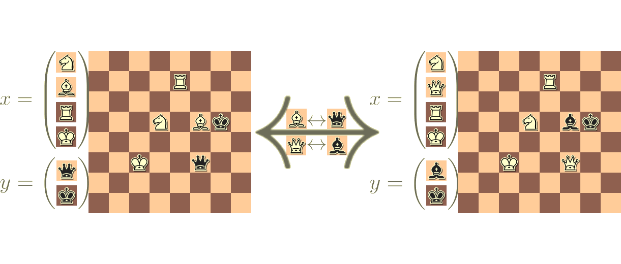
In contrast, the bilinear approximation is only invariant to reparametrizations of the strategy space of each player in isolation, but not to a reassignment of the decision variables accross players. Mathematically, we have
in general only if \(A = \begin{pmatrix} A_{xx} & 0\\ 0 & A_{yy} \end{pmatrix}\) is block-diagonal. Based on the above arguments, this is exactly the right set of invariances to be built into the approximation.
Reason 2: Bilinear plays well with quadratic regularization
One downside of Newton’s method in nonconvex optimization is that its update rule can amount to players choosing their local worst strategy if the critical point is a local maximum instead of a local minimum. This can be countered by adaptive choice of step sizes, trust-region methods, or cubic regularization, but a distinct benefit of first order methods is that their updates always amount to optimal strategies of the local game. Bilinear approximation preserves this important property while at the same time leading to an interactive local problem.
Reason 3: Fully exploiting first order regularity
Many competitive optimization problems have the structure
\[f(x,y) = \Phi\left(X(x), Y(y)\right),\] \[g(x,y) = \Theta\left(X(x), Y(y)\right),\]where the functions \(\Phi\) and \(\Theta\) are highly regular, but the functions \(x \mapsto X(x)\) and \(y \mapsto Y(y)\) might only have first order regularity. In the setting of GANs for instance, \(x \mapsto X(x) = \mathcal{G}_x\) maps the generator weights to the induced probability measure and \(y \mapsto Y(y) = \mathcal{D}_y\) maps the discriminator weights to the induced classifier. In the original GAN, \(\Phi\) would then be given as \(\Phi(\mathcal{G},\mathcal{D}) = \mathbb{E}_{z \sim \mathcal{P}}[\log(\mathcal{D}(z))] + \mathbb{E}_{z \sim \mathcal{G}}[\log\left(1 - \mathcal{D}(z)\right)]\). We observe that in this case the mixed derivative \(D_{xy}^2 f(x,y) = (D_{x}X) D_{XY}^2\Phi (D_{y} Y)^{\top}\) is well behaved, since only one derivative falls onto each \(X\) and \(Y\). The “pure” second derivatives \(D_{xx}^2 f\) and \(D_{yy}^2 f\) however require second order regularity of \(X\) or \(Y\). Thus, instead of requiring second order regularity, the bilinear approximation fully exploits the first order regularity present in many competitive optimization problems.
Does it work?
Gaussian mixture GAN
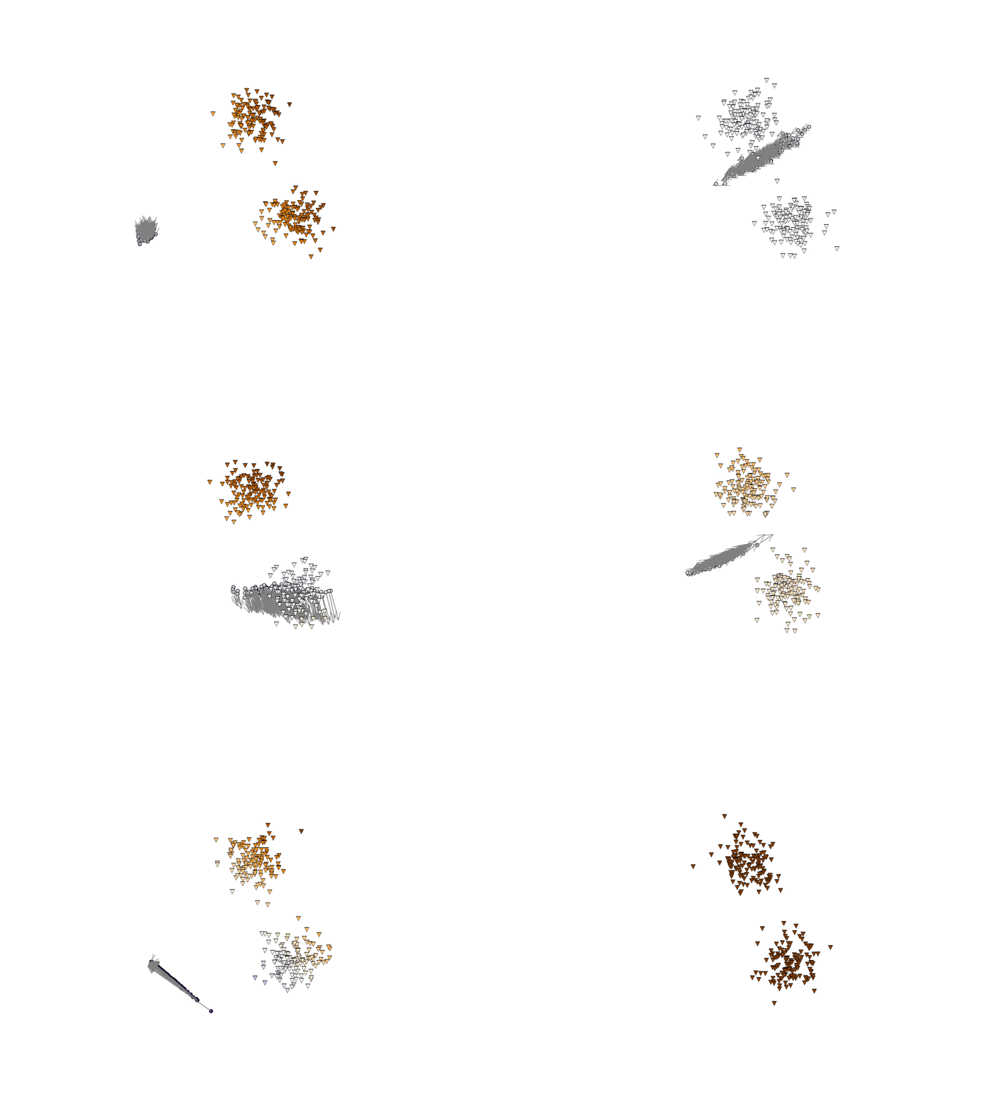
As a first experiment, we tried using CGD on GAN fitting a bimodal Gaussian mixture. While this is obviously a simple problem that can be solved with a variety of algorithms, it has the advantage that it lends itself to an easy visualization. With many of the existing methods we observed a strong cycling behavior with generator and discriminator chasing each other between the two modes. In contrast, throughout all step sizes that we tried, CGD seemed to show initial cycling behavior followed by a rapid splitting on the two modes. We emphasize that the other methods surely could be made work on this problem with the right hyperparameters. The main point of interest of these experiments is the sudden splitting of mass observed when using CGD.

Linear-quadratic GAN
In order to study the convergence speed of CGD, we consider a linear-quadratic covariance estimation problem given by the loss function
\[-g(V,W) = f(V,W) = \sum_{ij}W_{ij}\left(\Sigma_{ij} - \left(V V^{\top}\right)_{ij}\right)\]The main take-away is that while CGD has a higher cost per iteration than other methods, it is able to take larger steps without diverging, which often allows it to converge faster even when accounting for the Hessian vector products required for computing the matrix inverse in the CGD update using iterative methods.
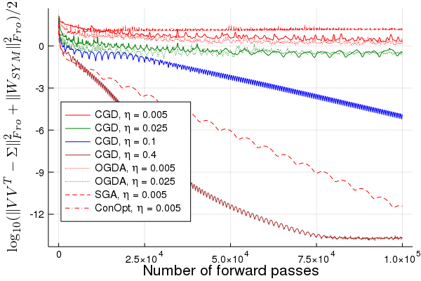
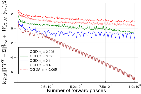
Image GANs on CIFAR10 and implicit competitive regularization
As part of a separate work, Hongkai, Anima, and I have investigated the performance of CGD on image GANs. For instance, we observe that when taking an existing implementation of WGAN-GP, removing the gradient penalty, and instead training with CGD, we obtain an improved inception score of CIFAR10! We explain this behavior with an implicit regularization induced by CGD. If you want to know more you should check out the paper or drop by the SGO & ML workshop this Saturday at Neurips. Of course there is still a lot to explore, so feel free to check out Hongkai’s pytorch implementation of CGD and try out CGD on your own problems!
CGD for equality constrained optimization
An important class of competitive optimization problems arises from equality constrained optimization problems
\[\min_{x \ : \ h(x) = 0} f(x)\]that can be rewritten as
\[\min_{x} \max_{\mu} f(x) + \mu^{\top} h(x)\]using a Lagrange multiplier \(\mu\).
Pierre-Luc, Clement, Anima, Emma, and I are presently investigating the effectiveness of CGD in the context of equality constrained optimization problems arising in reinforcement learning (RL) and control.
If you are interested to learn more, check out our workshop paper, the implementation using JAX, or our poster at the NeurIPS 2019 workshop on optimization for RL.
Conclusion
In the above, I have tried to convince you that CGD is indeed the natural generalization of gradient descent to two-player games.
In future posts and papers, I hope to comment in more detail on extensions to multiple players and higher order regularity, as well as the implicit regularization of CGD and how it can meaningfully stabilize GAN training even in the absence of Nash equilibria.